Overview

In this project, I implemented a perceptually realistic cloth simulator and built several shaders to broaden the artistic toolset available for stylizing the simulation. At a high-level, the cloth simulator is driven by equations of motion from classical mechanics and a dedicated cloth data structure. Conceptually, the cloth is modelled as a 2D grid of point masses connected by an isometric spring lattice. The motion of each point mass on the grid is governed by the cumulative effect of the spring forces (obeying Hooke's Law) and external forces. The simulation propagates the position of each point mass forward in time using Verlet Integration techniques. While there are energy losses in this technique, the simulator retains stability. As part of the simulator, I also addressed collisions with objects in the scene as well as self-collision effects to prevent the cloth from passing through itself. I was amazed that this simulator could present perceptually convincing cloth behavior with a variety of material effects while circumventing the computational costs of ray tracing - on my CPU the simulator worked in near real-time. I found myself deeply drawn to the underlying physics enabling these simulations. After extensively scrutinizing some of the unphysical conditions imposed for guaranteeing stability in the simulator, I found was able to reconcile such innaccuracy in the model physics with the perceptual accuracy of the simulator. I will remark on these justifications in the numerical integration section of the write-up.

Part I: Masses and Springs

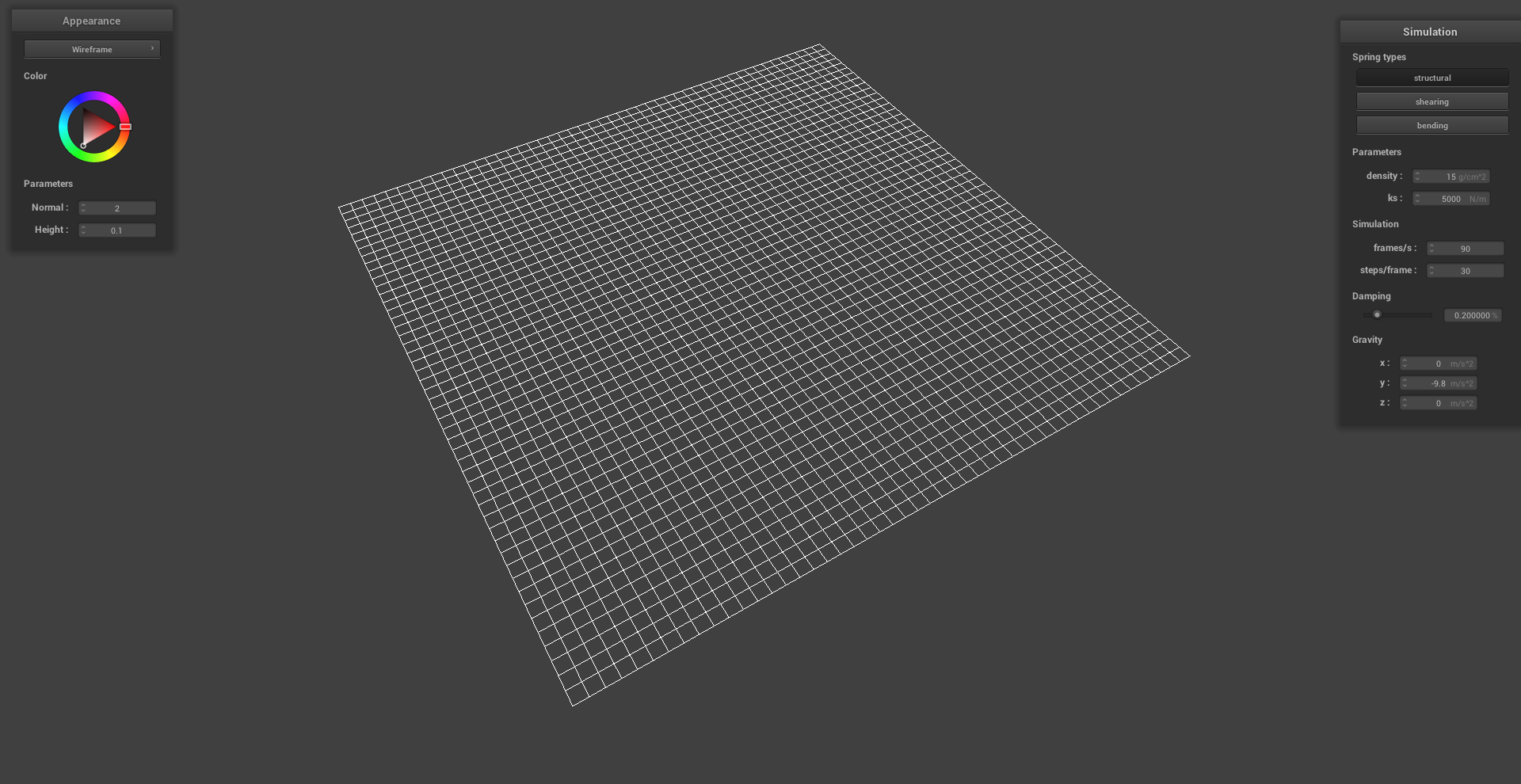
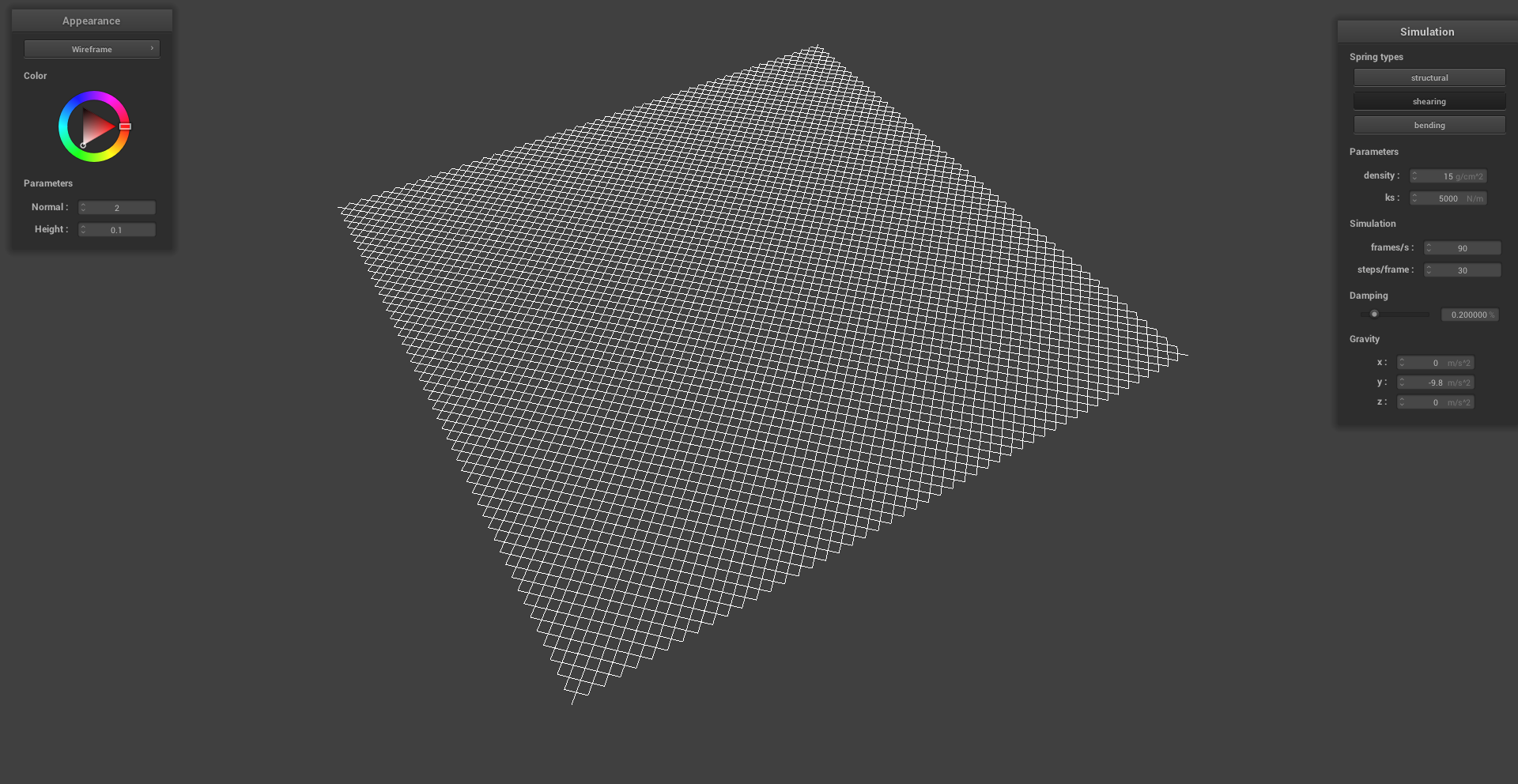
The cloth is modelled as a grid of point masses connected by an isometric lattice of springs. Additionally, each point mass has a "pinned" parameter which establishes whether or not the point mass will remain stationary throughout the simulation. There are three types of springs that we consider in our simulation: Structural, Shearing, and Bending. The first two offer isometric resistance to stretching and compression within the plane of the cloth. The bending springs supply resitance to deformation in the out-of-plane direction. The connective geometry of the structural and shear springs are shown side-by-side in the images below. For each of these spring types, we model the forces they introduce on the point masses using Hooke's Law. Central to this law is the notion of a rest length - the length of the spring at its lowest potential energy state. As such, each spring type has a different rest length based on its geometric orientation in the lattice. Suppose the structural springs have rest length \(L_0\). Then the shear and bending springs have rest lengths \( \sqrt{2}L_0 \) and \( 2L_0 \) respectively. As we can see in the images, the structural and bending springs align along the cartesian axes of the grid while the shearing springs align in the diagonal direction. Focusing our attention for a moment to the springs connection only to the immediate neighbors of a single point mass, any internal (non-edge) point mass in the grid has 8 springs attached radially. Thus displacement from an equilibrium position in any direction will invariably produce a near-isometric restoring force as though the point mass were positioned in parabolic potential well.

Part II: Simulation via Numerical Integration

Verlet Integration was central to position update procedure acting on each point masses in the cloth. In short, this method essentially runs Forward Euler and then retroactively imposes the unphysical constraint that the springs cannot extend beyond 10% of their rest length. This constraint is introduced to preserve the stability of the simulation but results in energy losses. There are two parametric quantities apparent in the equations of motion for our model that one can tune in the simulations: the spring constant \(k_s\) and the mass (i.e. the density toggle in the simulator). Additionally, there is a third tunable parameter that is not explicit in the equations of motion for our model: damping. We introduce damping to further stabilize the simulation and ensure that the cloth eventually comes to rest. Below I visually demonstrate how these parameters affect the cloth simulation by adjusting each parameter independently.

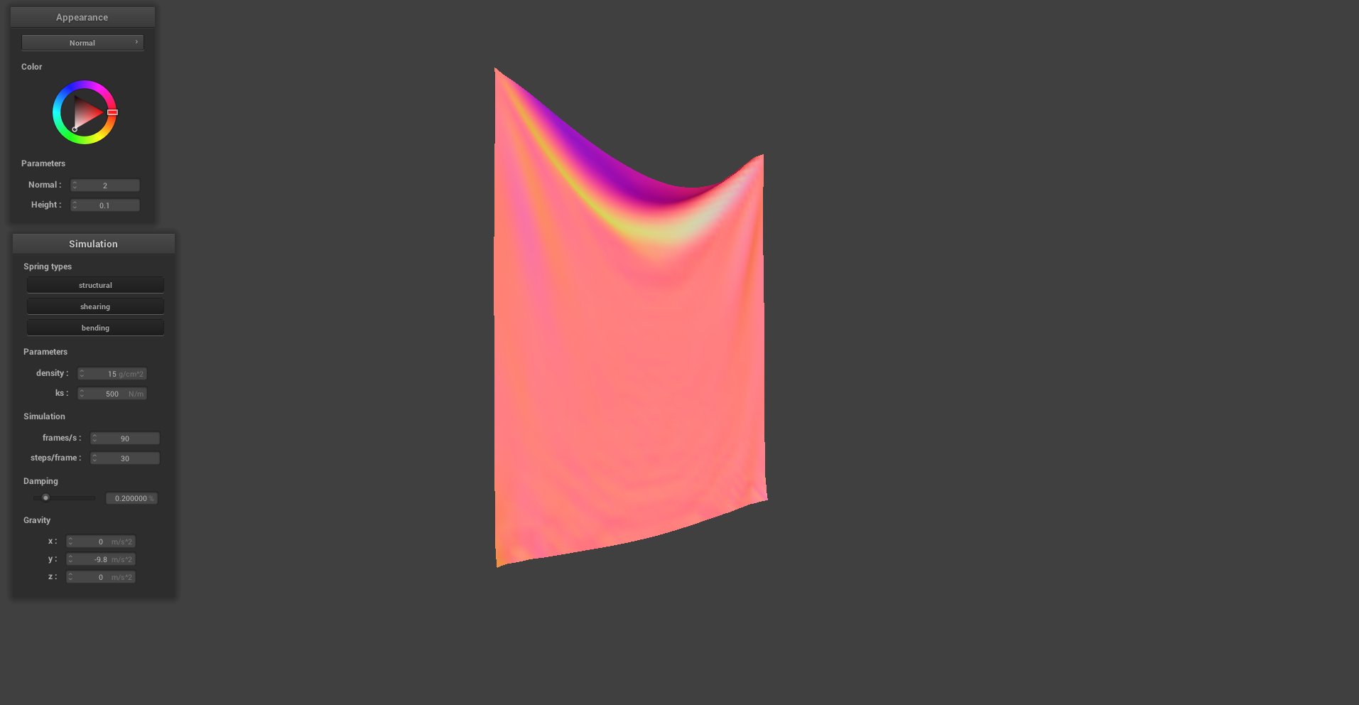
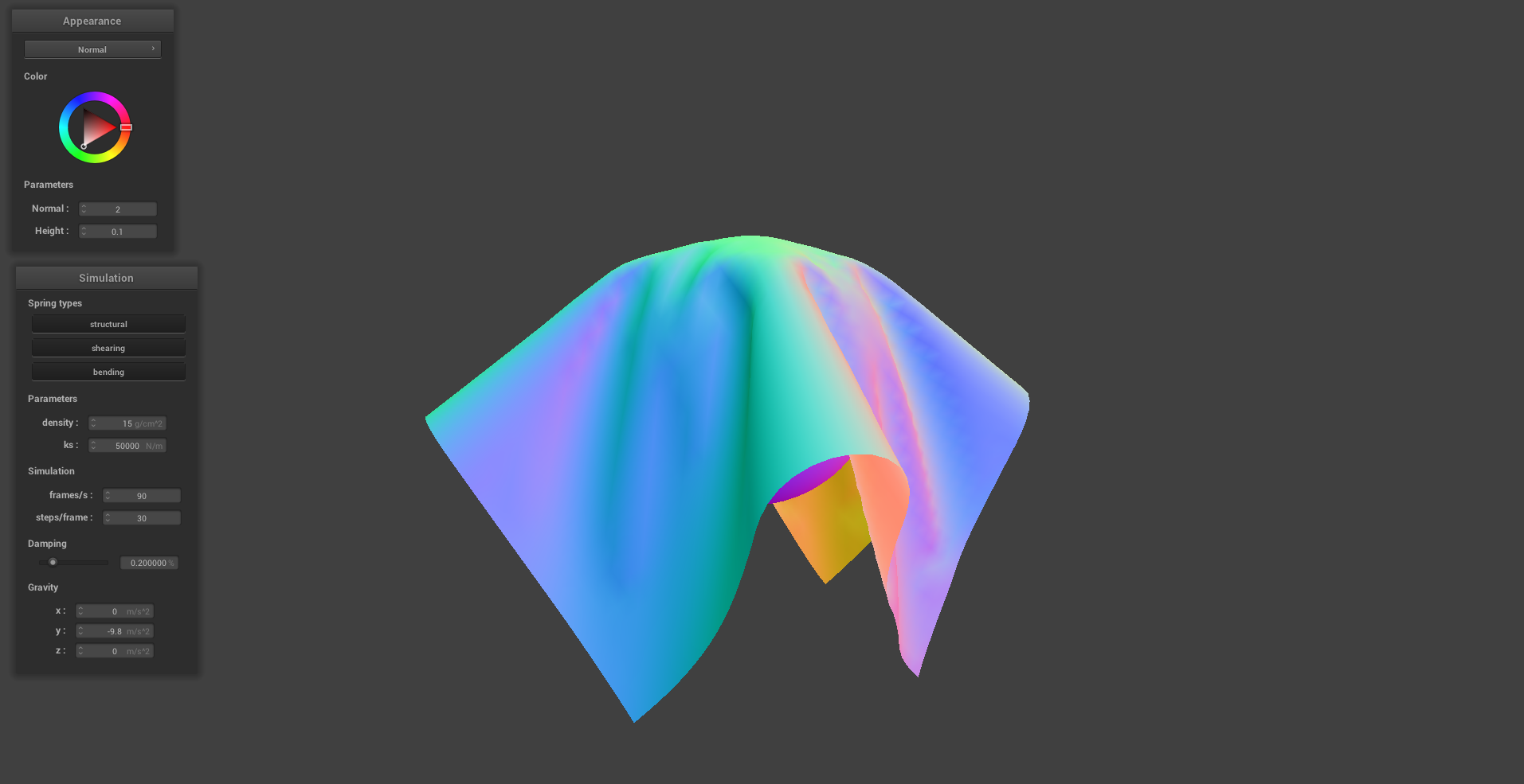
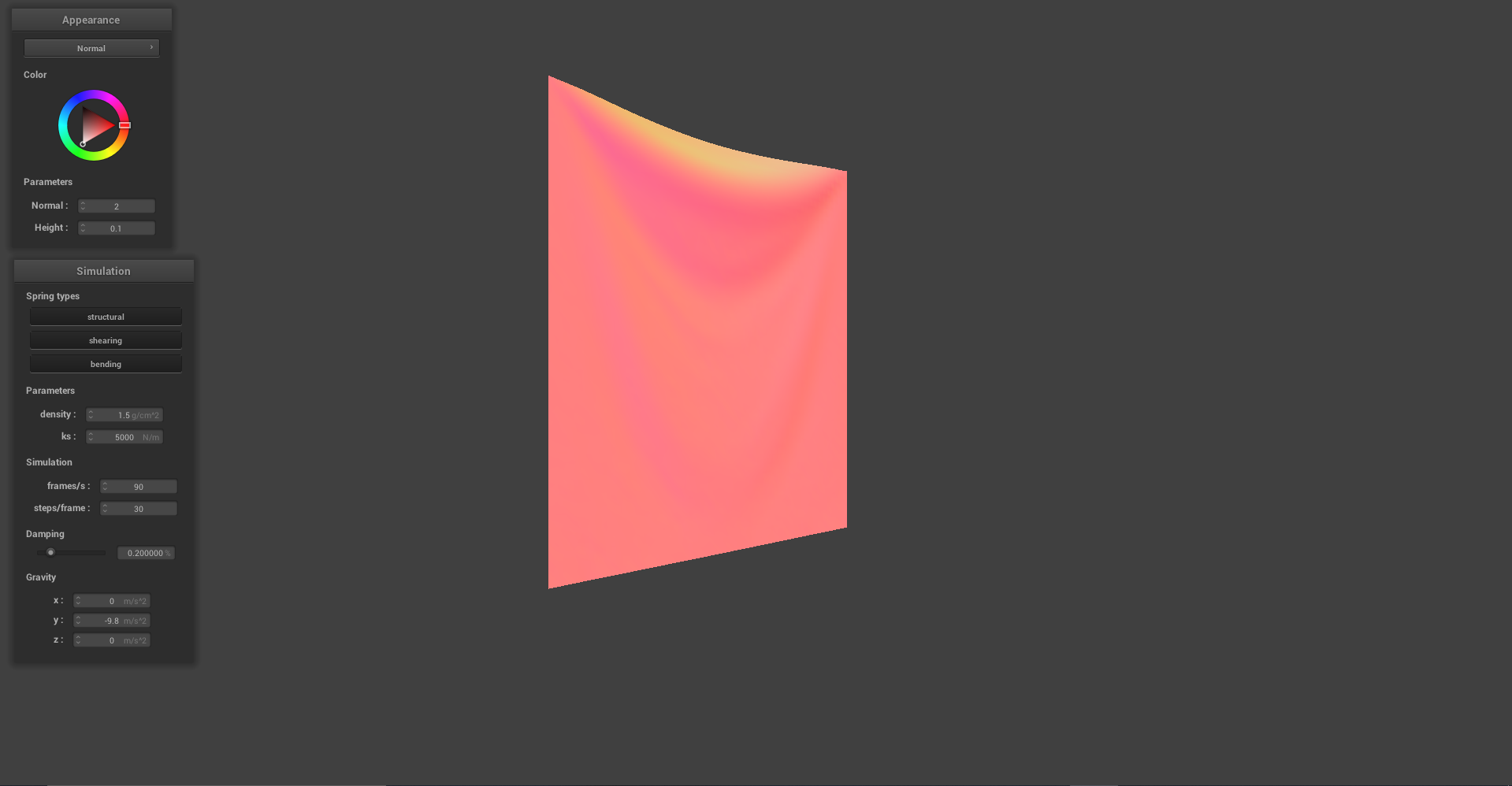
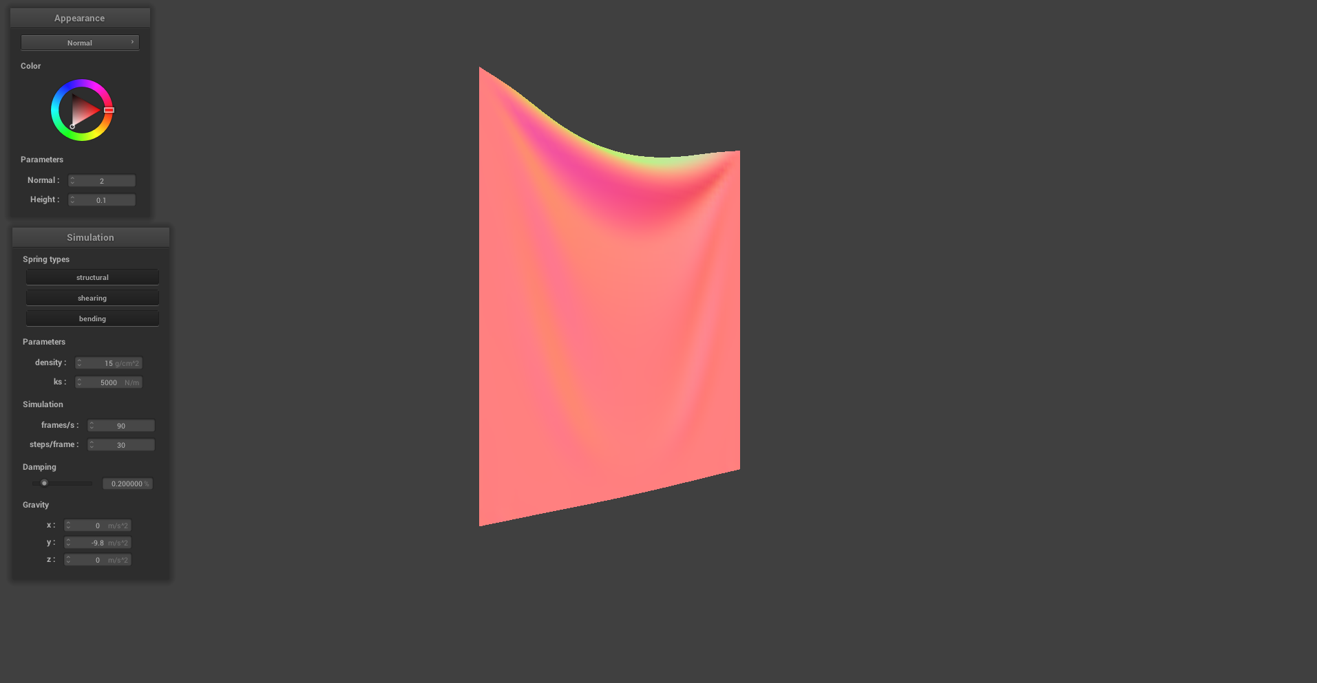
SPRING CONSTANT:

Increasing the spring constant effectively increases the spring's stiffness. Scanning the images below from left to right, we see the spring constant drop by two orders of magnitude. The cloth appears to become more maleable for lower spring constants as stretching is more drastic for the \( k_s = 500 N/m \) case compared to the \( k_s = 50,000 N/m \) case even though both simulation environments featured the same gravitational field.

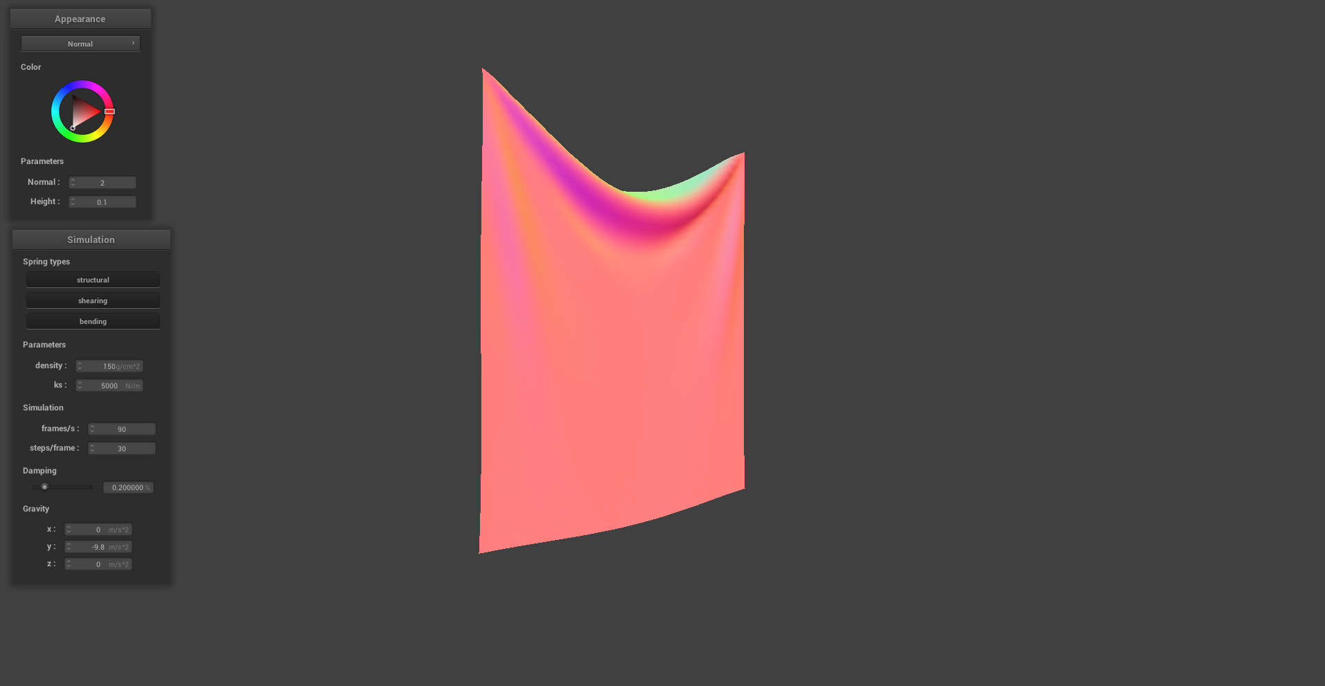
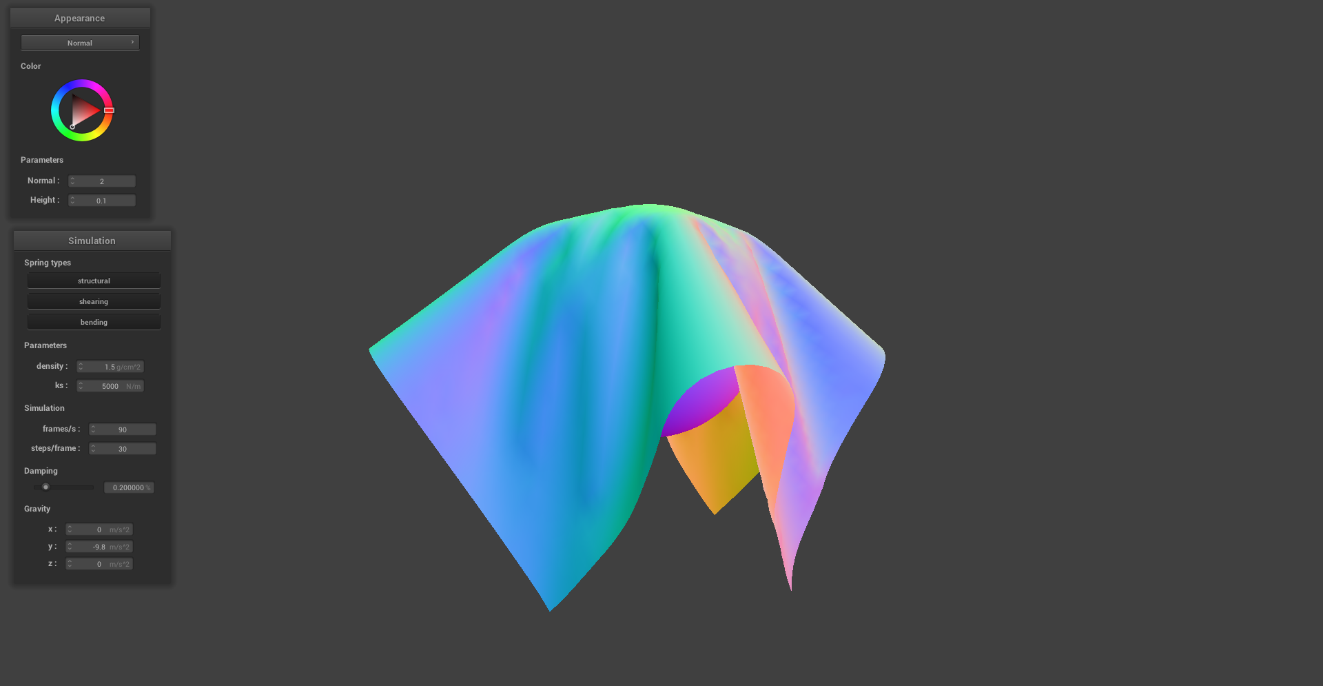
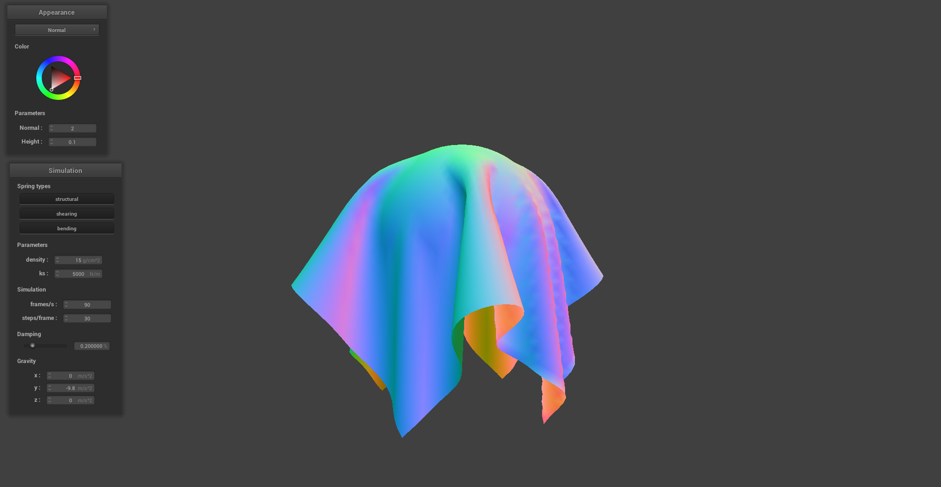
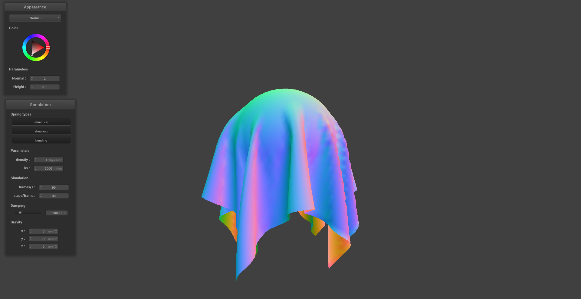
DENSITY:

The density is attribute of the point masses rather than the springs. Increasing the density has a similar effect on the cloth compared to decreasing the spring constant. This similarity can be explained through Newton's Second Law which posits that a force on an object is proportional to its mass. Thus the cloth is more susceptible to the external forces in the simulation, namely gravity.

DAMPING:

The effect of damping is somewhat less evident in still imagery. However I noticed in live simulations that the damping value greatly affects how quickly the simulation reaches a state of rest. Higher damping values cause the simulation to come to rest more rapidly. The two images shown were taken after long integration times. The image on the left is of a simulation with 0% damping. Here, the cloth never reaches a state of rest as illustrated by the small perturbations/oscillations that persist in the cloth even after long integration times (It may require zooming in to see these). The image on the right is of a simulation with 1% damping. Here the cloth is completely at rest as seen by the smooth contours of the cloth.

PINNED CORNERS:

Reflections on Moments of Confusion:

While implementing Verlet Integration, I contrived an edge case in which the repositioning of the point masses (i.e. limiting the spring extension to be less than 10% of the rest length) does not solve the issue of overextension. Suppose two springs are attached to opposite sides (say the left and right sides) of point mass. Further, suppose that the left spring is overextended while the right spring is not. In moving the point mass to the left to correct for the overextension, it is possible that the right spring becomes overextended in this process. Upon realizing this, I placed the retroactive Verlet step in a loop that continues to readjust the cloth until there are no overextended springs remaining or a maximum number of iterations is reached. However, this seriously slowed the simulation down with no visible improvements to the simulation quality. Therefore, I returned to applying the overextension correction only once per time step. Separately, when I first encountered Verlet Integration the approach did not sit well with me. Setting a hard limit on the maximum extension of the spring seemed like a highly unphysical constraint. Consequently, I was as amazed as I was perplexed to see how preceptually convincing the simulations were. In looking into this further, I realized that there is a semi-convincing justification behind imposing this constraint that is grounded in realistic physics. For many materials, the spring coefficient is itself a function of the displacement from the rest length. In this regard, imposing the maximum extension limit for Verlet integration has similar behavior to a spring constant that increases exponentially with respect to the departure from the rest length.

Part III: Handling Collisions with Other Objects

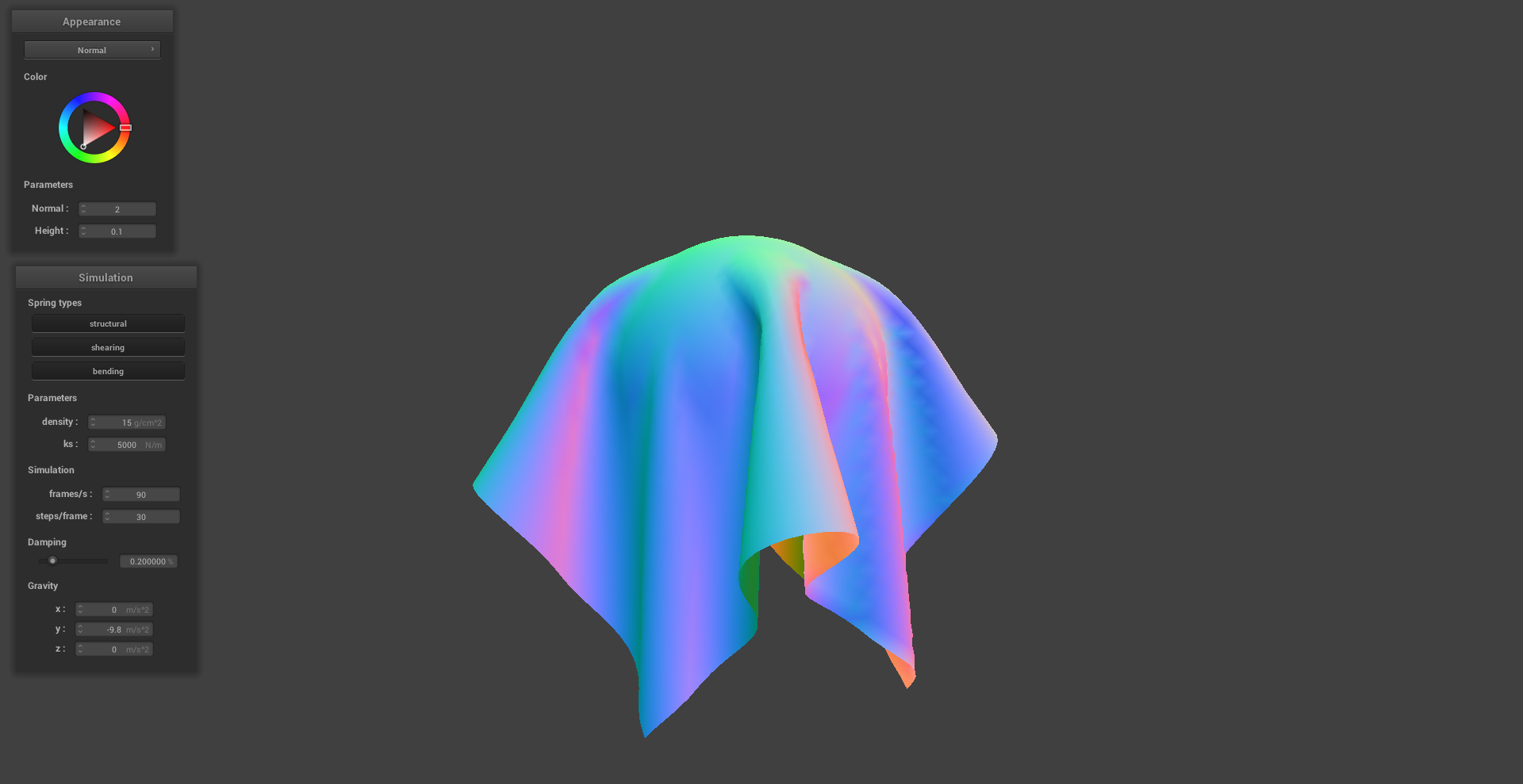
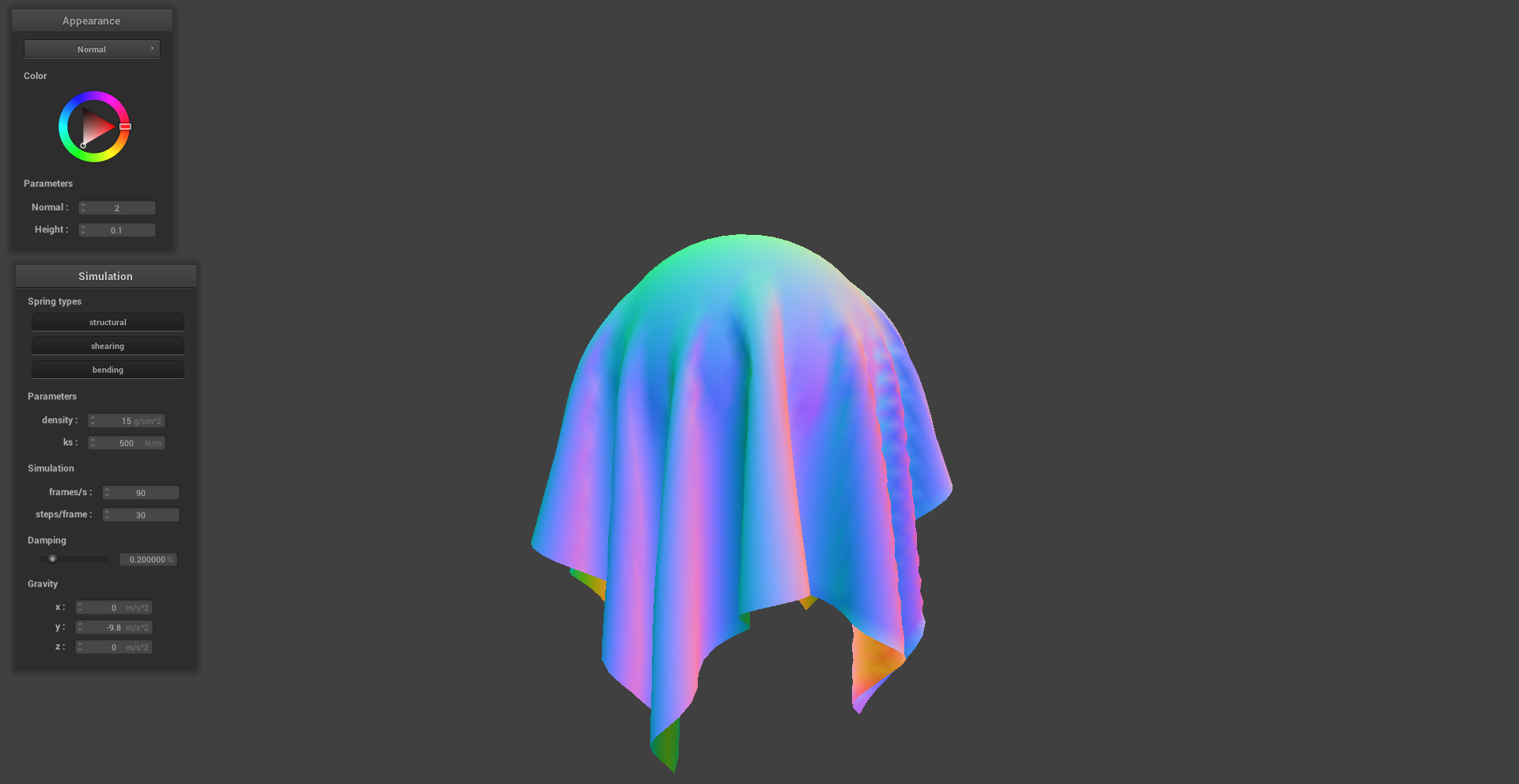
To simulate collisions with other primitive objects (i.e. the plane and the sphere), I exploited the implicit vector definition of their geometries to identify where the cloth crossed the surface boundary of the primitives. The images below demonstrate the cloth interacting and colliding with these primitives. As we can see, in the sphere collision image the cloth conforms only to the top half of the sphere. This is because the points where the cloth is in contact with the sphere experience a normal force conteracting the external gravitational force present in the simulation environment.

Part IV: Handling Self-Collisions

For performance purposes we take advantage of the fact that self-collisions must occur locally. In other words, two point masses on opposite ends of the world environment will never collide, but two within a small voxel may. This means we can divide 3D space into a volumetric grid and bin each point mass into one of the cells. Then the self intersection checks on the cloth only have to be performed between point masses contained within the same cell. Using a hashmap whose keys are generated using the discrete voxel coordinates, we have an adaptive data structure that stores all the point masses within a certain vicinity of one another. Ideally, the hashing function introduces very few collisions throughout the simulation (i.e. no two voxels map to the same key). For my implementation I used the following hashing function. Here \(\bar{x},\bar{y},\bar{z}\) are the integer coordinates of the voxel.

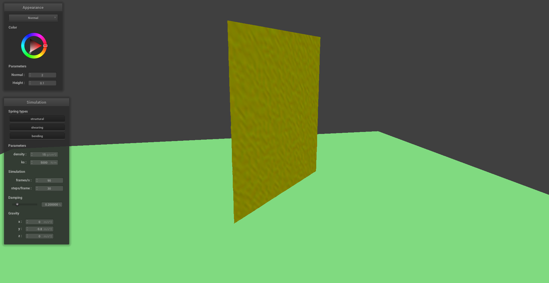
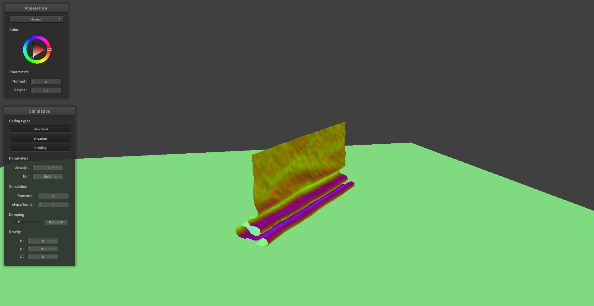
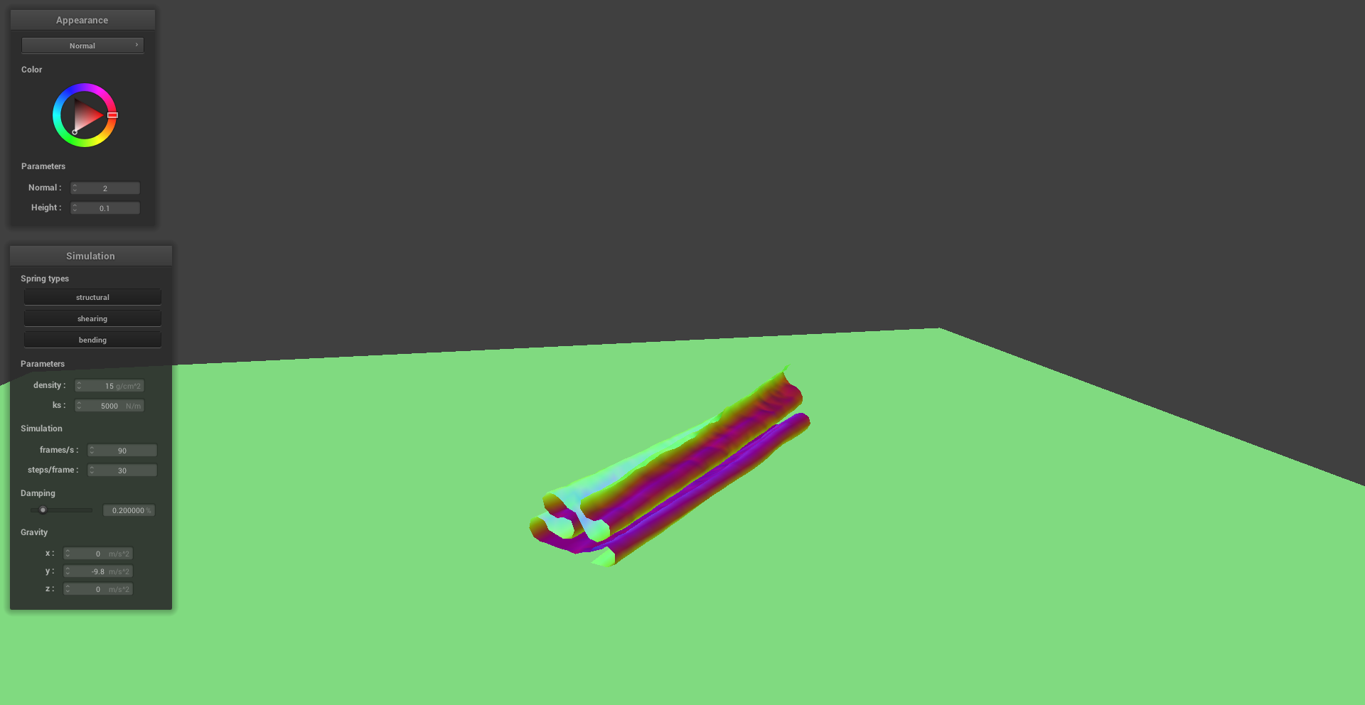
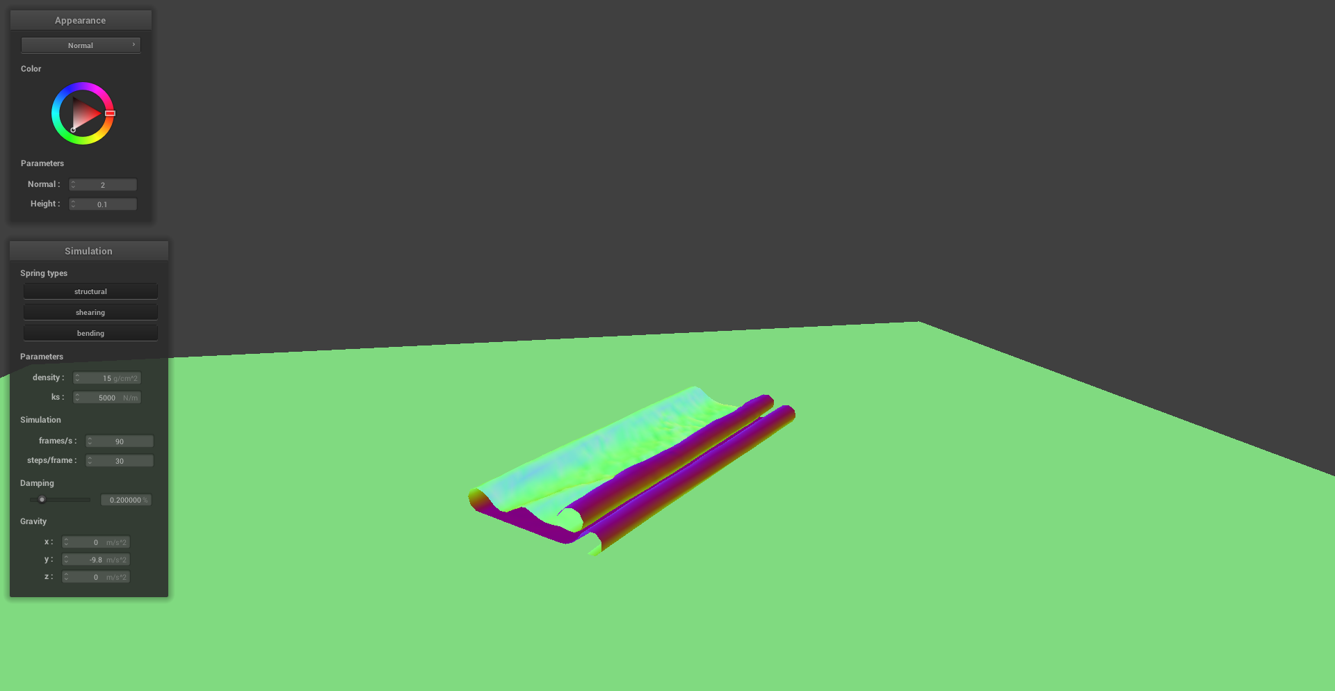
\begin{equation} \text{hash} = \bar{x} + \bar{y}^2 + \bar{z}^3 \end{equation}

The image sequence below depicts snapshots of a cloth simulation performed over a time T. The snapshots were captured at equally-spaced time intervals and demonstrate how the cloth is self-avoiding and does not self-intersect. Specifically, we see that no two sections of the cloth ever completely come into contact with one another. This can be attributed to an internal cloth thickness parameter in the implementation which imposes a hard limit on how close two point-masses can ever be from one another throughout the simulation.

Part V: Shaders

Shader programs in GLSL offer a computationally inexepensive alternative to rendering realistic material appearances without exhaustive ray tracing. Shader programs are built in two parts: 1) A vertex shader - which assigns vertex attributes in the scene and transforms the scene to normalized device coordinates. 2) A fragment shader - which assigns an RGB-alpha vector for each pixel in the display based on interpolated vertex data. Data contained in the vertex attributes are manipulated in the fragment shader to produce different material effects. After the pixel values corresponding to each vertex are determined (since every vertex maps to a single pixel), the fragment shader interpolates between the known pixel values aligning with a vertex to fill in the remaining pixels.

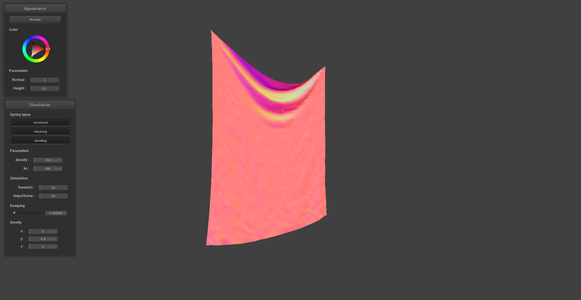
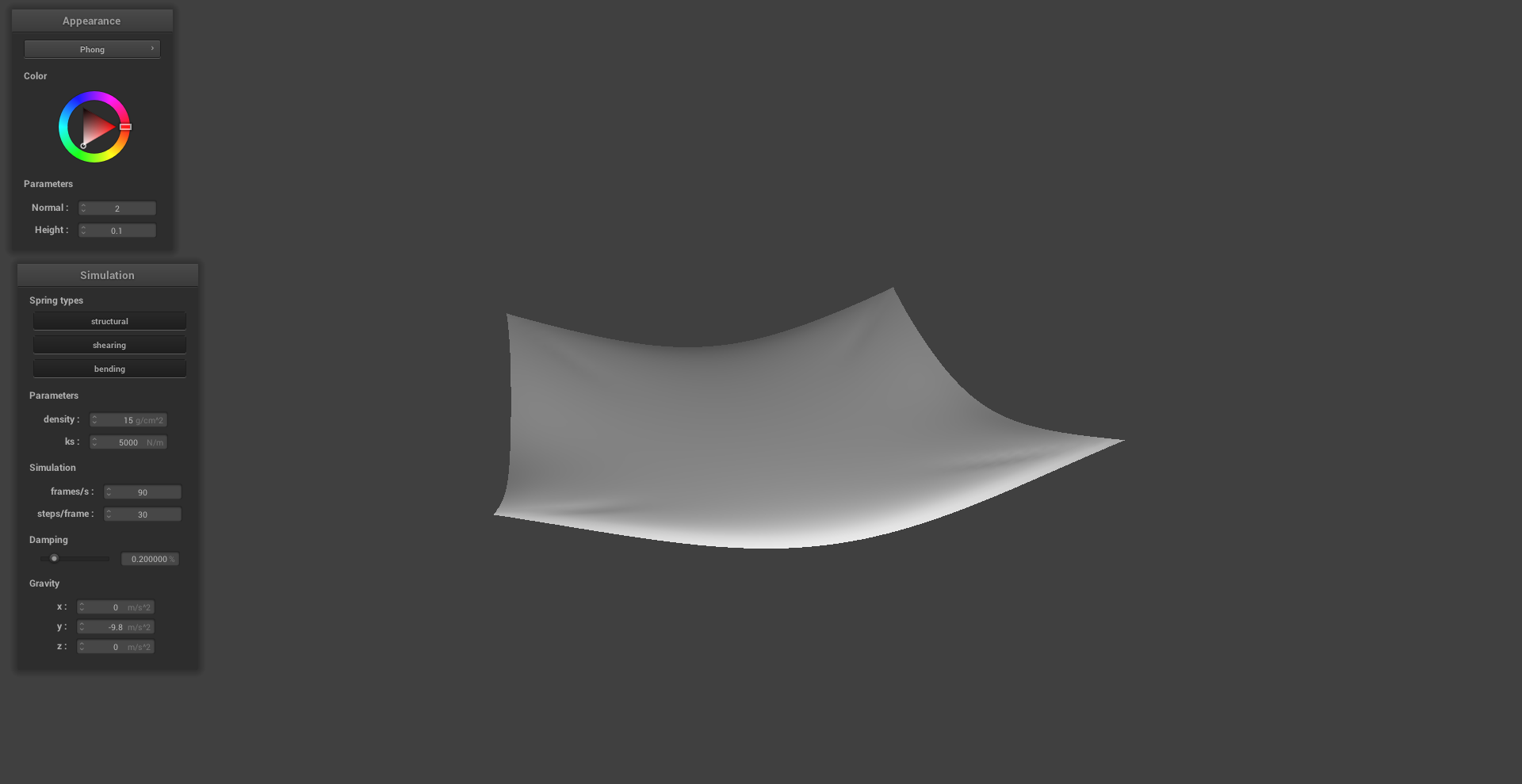
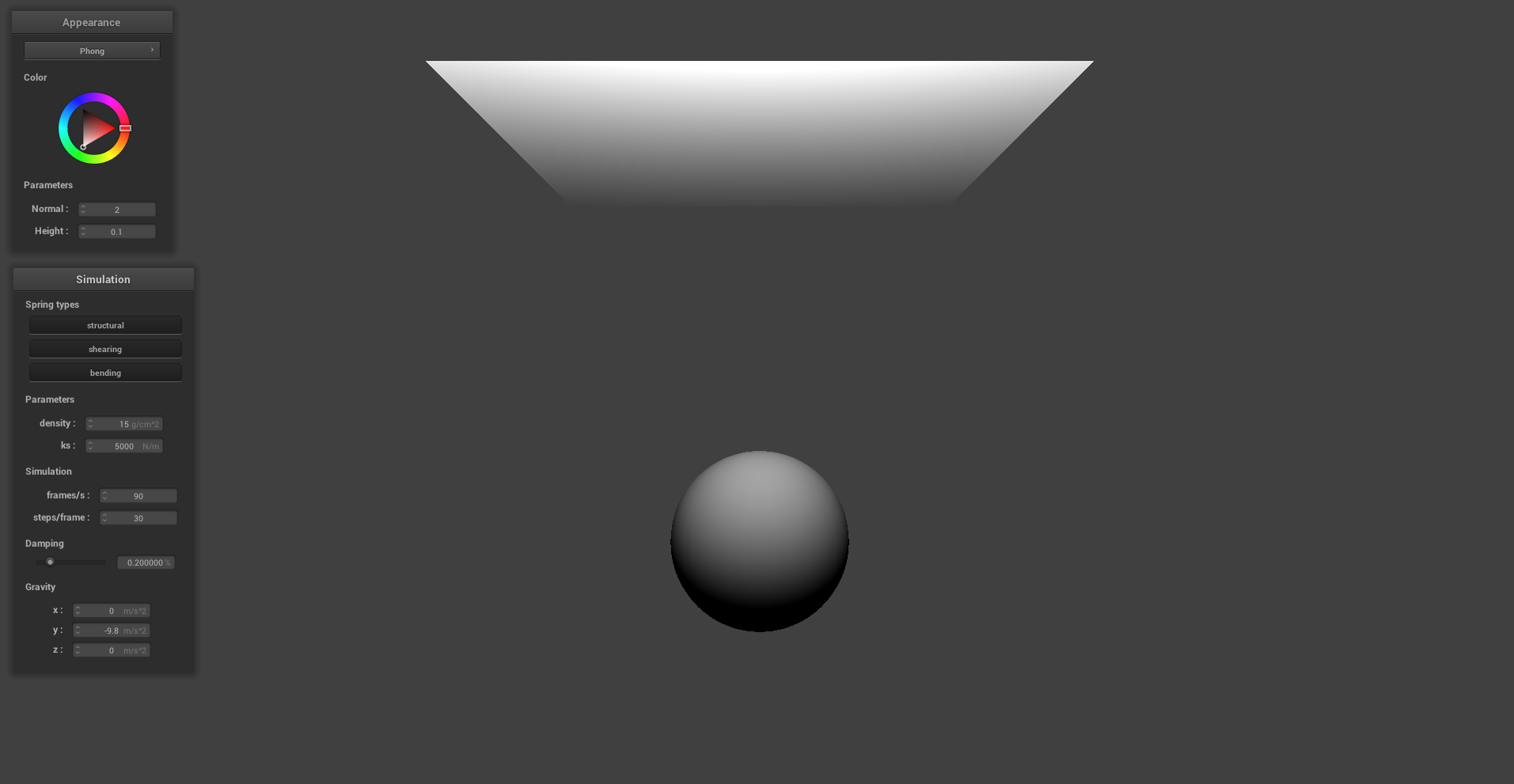
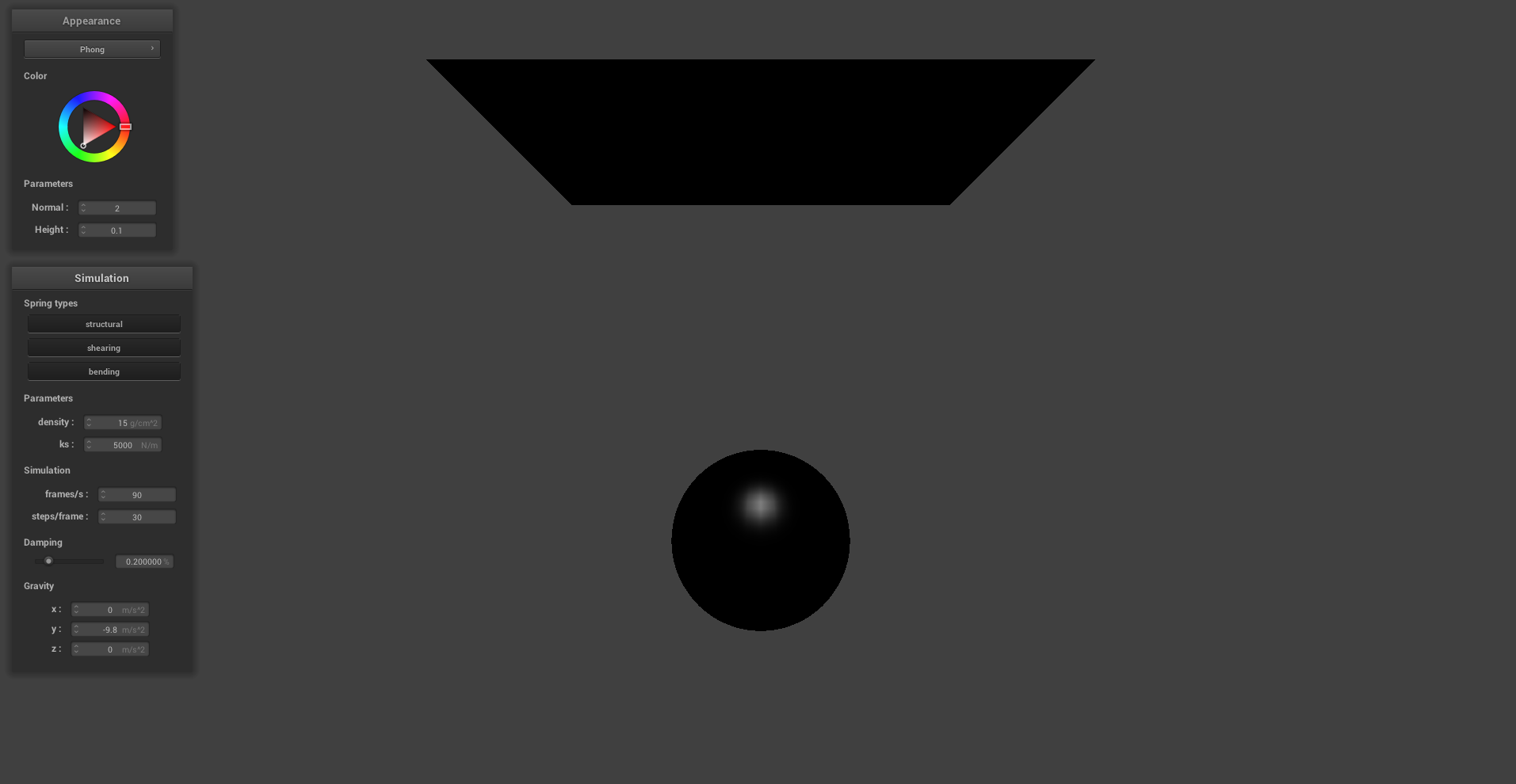
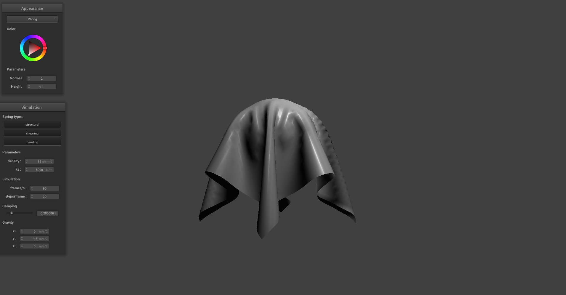
BLINN-PHONG SHADING:

The Blinn-Phong Shading model considers light contributions of three different types: the ambient light, diffuse light, and specular reflections. Ambient light can be thought of as the DC intensity reflecting uniformly off of all objects in the scene. Diffuser lighting is the a function of the local surface normal relative to the illumination source. Using Lamberts cosine law, the surface normals that point closer to the light source are those with the highest intensties. Finally, specular reflection relates the illumination source position, the surface normal, and the viewing position to produce a glare characteristic of glossy materials. The images below demonstrate each of these contributions in isolation while the final image poses them as a weighted sum. Depending on the weights of each contribution, we can simulate the appearance of different materials.

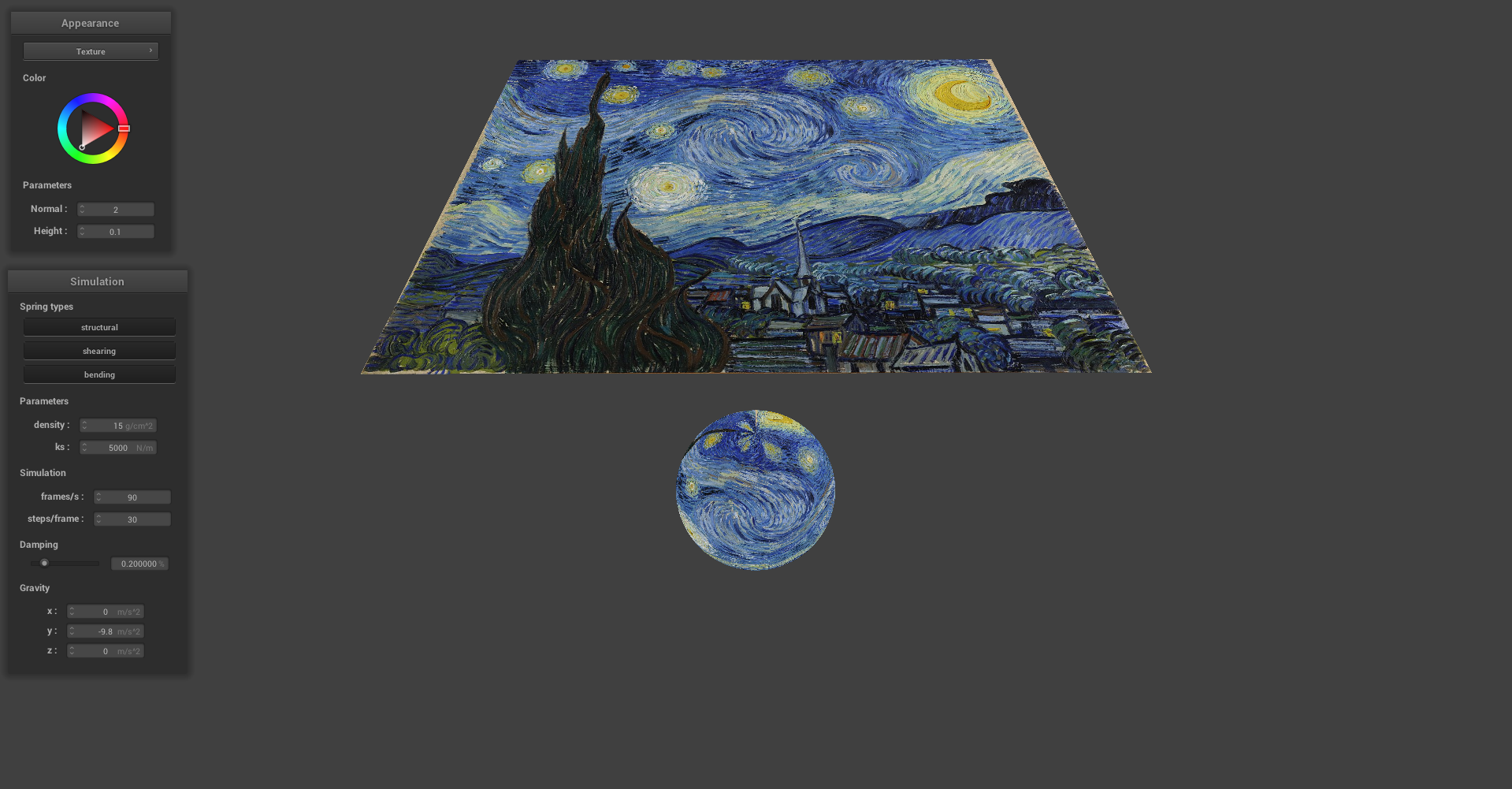
CUSTOM TEXTURE:

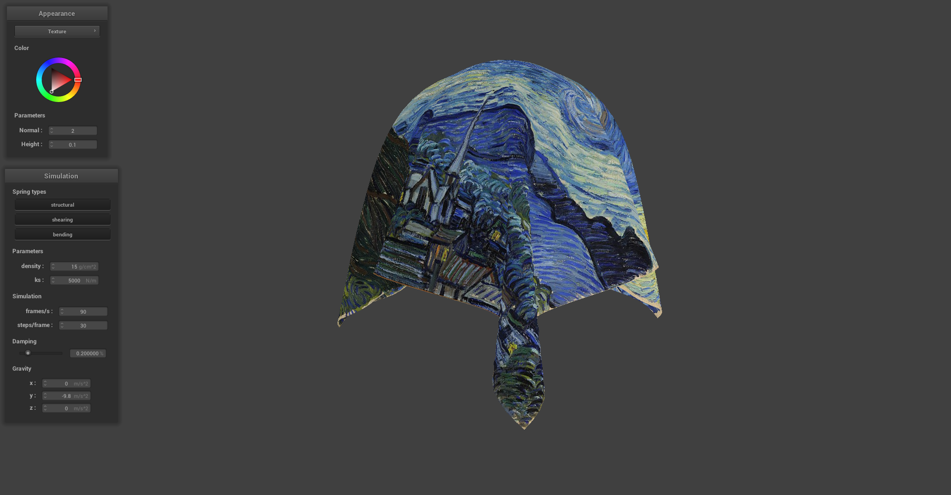
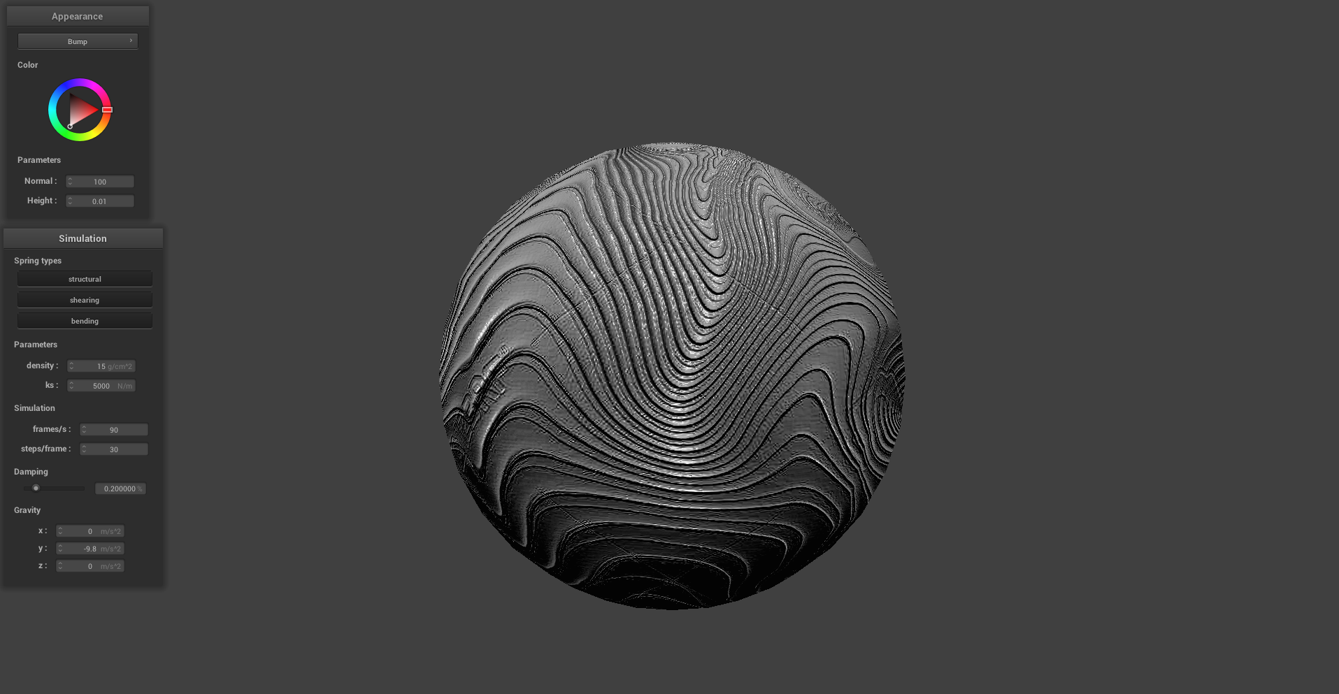
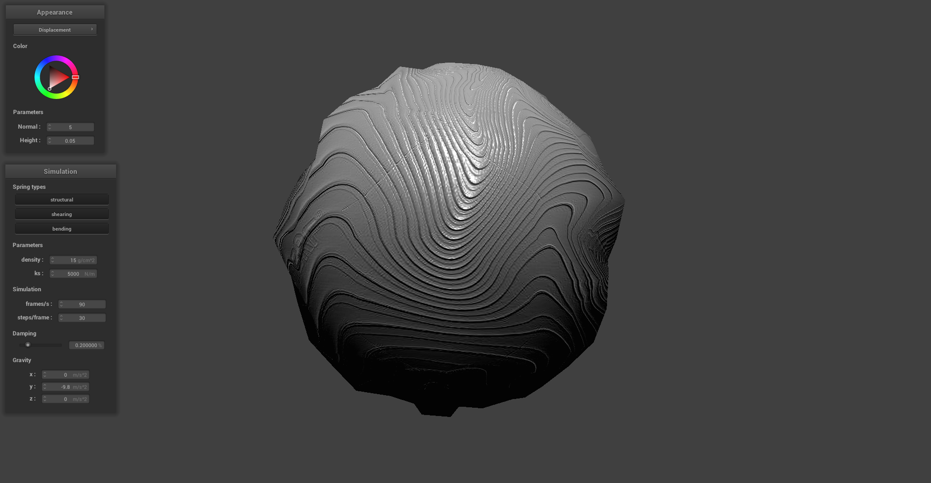
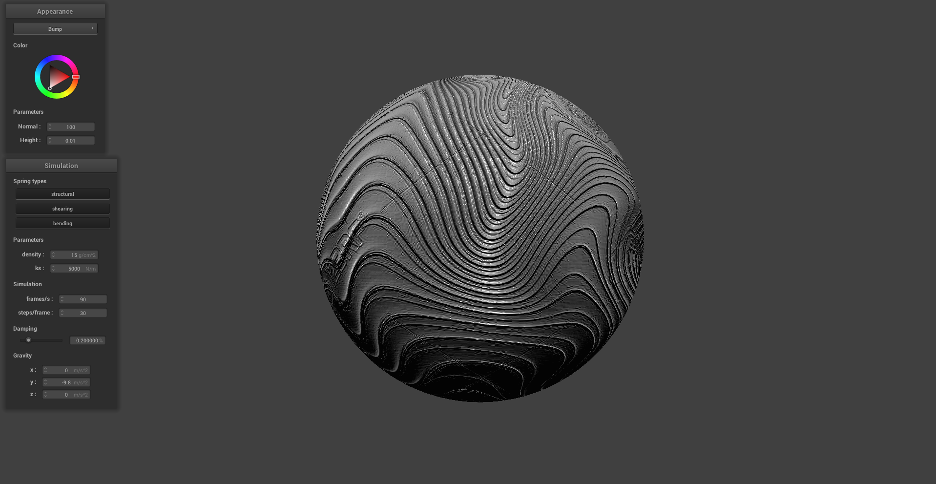
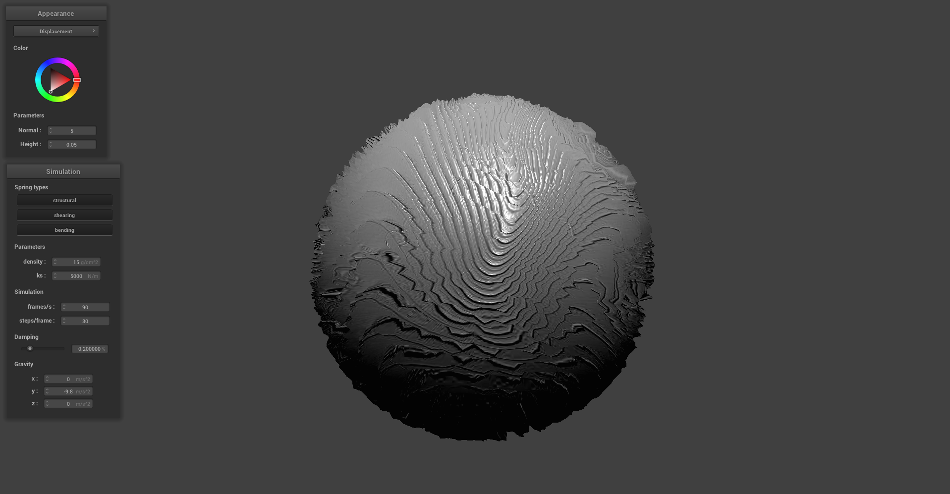
BUMP AND DISPLACEMENT MAPS:

The images below show bump mapping and displacement mapping of a texture on a sphere. For the first row of images, the surface of the sphere is sampled at 16 lateral and 16 longitudinal coordinates for a total of 16x16 vertices. Visually, bump mapping seems to perform better than displacement mapping for this low sampling rate. This is clear from the strange blockiness of the sphere evident in the 16x16 displacement mapping image. Such blockiness appears because the fragment shader is interpolating physical height perturbations over the sphere from a relatively sparse number of samples. Meanwhile, the texture itself has ample high frequency content over the sphere that cannot be matched by the surface displacements due to the low sampling rate. In contrast, the second row features 128x128 samples on the sphere which is a high enough sampling rate for the surface displacements to match the high frequency content of the texture.In this case, we can see that displacement mapping accurately portrays both the shading of the texture as well as the physical deformations on the sphere defined by the texture.

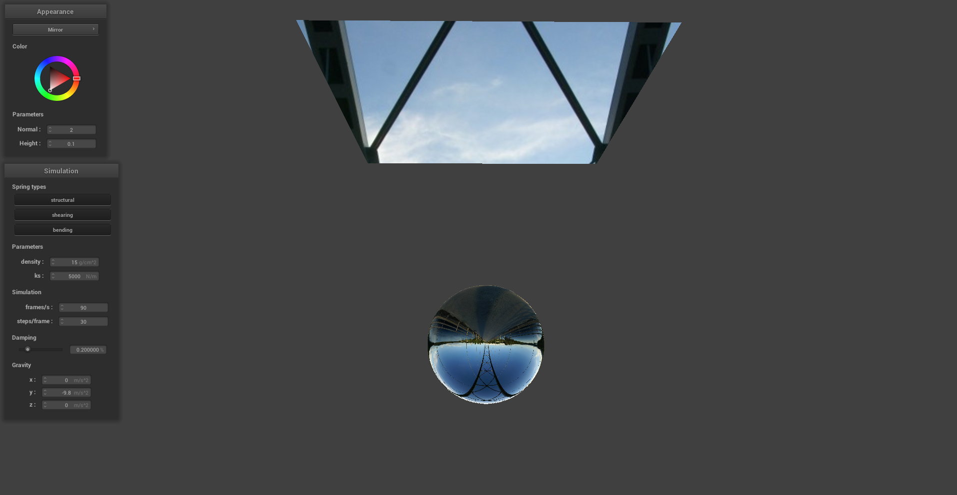
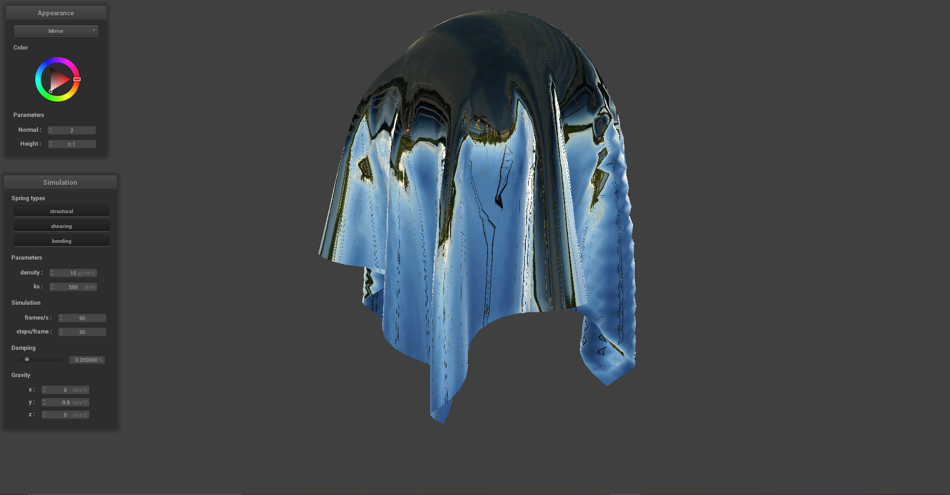
MIRROR SHADER: